8.4 Sampling Distribution
Consider a finite population of 4000 students of a certain college. Of this 200 students are selected randomly and their mean weight is calculated. It was computed as x = 135 lbs. If we draw 20 different samples of 200 students, instead of just one as we did previously. We cant expect the same mean weight of these 20 samples chosen randomly. It is due to sampling variability i.e. each sample drawn randomly from the same population differs from each other in their computed 'statistic'.
The means computed is listed as
|
130 |
137 |
140 |
131 |
132 |
133 |
128 |
125 |
129 |
138 |
|
133 |
134 |
142 |
145 |
136 |
134 |
128 |
143 |
137 |
136 |
These 20 values form what is known as a part of the sampling distribution of a statistic "mean" weight. Therefore, the sampling distribution is the statistic calculated for a large number of random samples drawn from the same population.
Alternatively, consider all possible samples of size 'n' which can be drawn randomly from the same population, and for each one, compute the aimed statistic. In this manner we obtain the distribution of the statistic, which is the sampling distribution.
Now we compute mean of this sampling distribution which is 134.55 lb (note that is obtained using the formula 
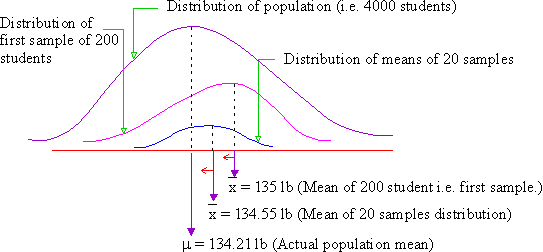
Now we are told that the population mean ( m ) i.e. mean weight of 4000 students is 134.21 lb (In case of infinite population, this is not known). Therefore, 135 lb is not a bad estimate of the population mean. But 134.55 lb is a still better estimation. We thus conclude that the more the sample means (statistics) included in the sampling distribution, the more correct the chances of the mean of the sampling distribution becoming an estimate of the population mean (parameter). The following graphical representation supports this argument.
 Click here to enlarge
Now recall the list of means computed for 20 random samples.
We observe that the 20 sample means differed form the true population
mean m = 134.21 lbs. The means 137, 140, 138, 133, 142, 142, 136,
143, 147, 136 are clearly above the true mean while 130, 131, 133,
132, 128, 125, 129, 133, 134, 134, 128 are below the true mean.
These deviations or differences from true value is due to the variability
of samples. This is known as 'Random error' in statistical estimation.
Note that the mean of 20 random sample means is slightly greater
than the true population mean. If we take 20 more samples of 200
students, the mean of this new sampling distribution might be lower
than the true population mean.
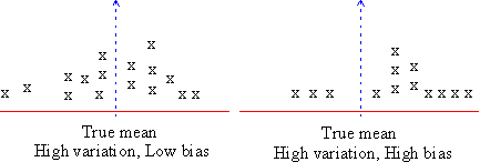
Other than random error, error arises due to the tendency of consistent under estimating or over estimating a true value. This is known as systematic error or bias. Suppose, in the example discussed above, an investigator is investigating only those students who are healthy and fit. He would most likely overestimate the population mean. Generally healthy bodies have reasonable weights. Clearly the investigator's choice is one of bias.
This is an example from one of the bias that occurs in estimation.

Click here to enlarge

Click here to enlarge
|