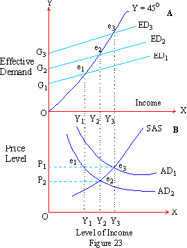
(H) Rigid wage rates and unemployment: Under the classical model as a rule there is no general and involuntary unemployment. Moreover, if there is some deficiency in demand and consequent unemployment in certain sections of the economy, it can at once be cured with the help of a cut in the wage rates. Keynes does not accept flexible wage rate as a solution to the unemployment problem. His chief argument in this respect is that workers are under money illusion. Therefore they strongly resist any attempt to cut down money wage rates. Moreover the working class is well organized and trade unions will thwart any such efforts (as wage cuts) on the part of employers. Therefore a cut in wage rate will not be possible and hence there will be a persistent unemployment condition. Let’s present this with the help of a figure containing aggregate demand and aggregate supply curves.

 

 

There are two parts of figure 23. In the upper part (A) is shown Effective Demand Curves generating real income levels. In the lower part (B) we find AD and SAS curves together determining levels of income and price levels. Let’s begin with part A where levels of income have been measured along the horizontal axis and levels of Effective Demand along the vertical axis. In this part of the figure there are three curves ED₁, ED₂ and ED₃ intersecting line OY at three points of equilibrium e₁, e₂ and e₃. Corresponding to the three levels of Effective Demand we have the sizes of autonomous public expenditure G₁, G₂and G₃ respectively. In the three equilibrium positions, the levels of income generated are Y₁, Y₂ and Y₃.

We have extended the vertical lines e₁Y₁, e₂Y₂, and e₃Y₃ downward to show the equivalent levels of income in part B. In this part, income levels have been shown along the horizontal axis as before, but this time along the vertical axis, price levels are indicated. AD₁ and SAS are the original aggregate demand and supply curves and AD₂ is the downward shifted aggregate demand curve. It would be appropriate to begin with point e₃ in part A which is the highest equilibrium point close to the full employment level. The corresponding point in part B shows point of intersection between AD₁and SAS. This determines initial level of income as Y₃ and level of prices as P₁. If for some reason autonomous investment is reduced and or for some other reason, effective demand level slides down from Y₃ to Y₁with new equilibrium position e1in part A. Then the level of income in part B will also appear to have reduced to Y₁ but it is not an equilibrium level between AD₁ and SAS curves.

As a result of a fall in the effective demand, the AD curve will shift down from AD₁ to AD₂. This helps to establish new equilibrium point e₂ which is the point of intersection between AD₂ and SAS. At this point the level of income established is Y₂ and the corresponding price level is P₂. With a fall in the price level, cost of production must have reduced to some extent which must have enabled produces to increase output from Y₁ to Y₂. Yet Y₂ output level is lower than Y₃ and at which there is some unemployment of labor. Under Keynesian model this unemployment is persistent and cannot be cured by the wage cut solution. The wage rate being rigid it cannot be cut down and hence SAS curve will not shift downwards to ensure full employment. However, equilibrium can be brought back to the original level e₃ and level of employment can be restored by avoiding unemployment. This becomes possible only through an upward shift in the effective demand curve with the help of additional public expenditure, increasing it from G₂ to G₃ (Part A). Keynes’ solution to unemployment is therefore in the form of an appropriate fiscal policy and adjustments in the public expenditure. This has been offered in order to increase effective demand substantially and that way, to maintain a sufficiently high employment level.

Index

5. 1 Classical Theory
5. 2 Keynes' Employment Theory

Chapter 6